Linear Analog Modelling - Steiner-Parker Filter [ C++ JUCE ]

 

    In this post, I'll delve into a method for modelling linear circuits. By linear circuits, I'm referring to circuits  composed of linear components such as resistors, capacitors, and inductors. This technique isn't applicable to circuits containing non-linear components like diodes or transistors. 

    For demostration I'll construct a Steiner - Parker low pass filter. 

 Analog Modelling 

    

    The technique employed for modelling involves extracting the differential equations that describe the circuit's behavior. Subsequently, numerical methods for solving Ordinary Differential Equations (ODE) are utilized to approximate the solution. 

    Equations for your circuit can be obtained either manually or with the assistance of software tools. In my case, I prefer using System Modeler and Mathematica (from Wolfram).        This approach proves particularly beneficial when dealing with intricate circuits where manual modification of component values or topology can become complex. 

 Challenges in Modeling Non-Linear Networks

    When dealing with non-linear components like diodes, solving equations in terms of output voltage becomes challenging. The non-linear nature, often involving exponential terms, results in implicit equations without symbolic solutions. Consequently, the only viable approach is numerical solutions, employing methods such as Newton-Raphson. Unfortunately, this numerical approach introduces a lot of latency to the process. 

    The realm of non-linear modelling in audio is expansive, offering a plethora of approaches. One notable method involves the use of black box models, particularly neural networks.

 Steiner Parker topology 

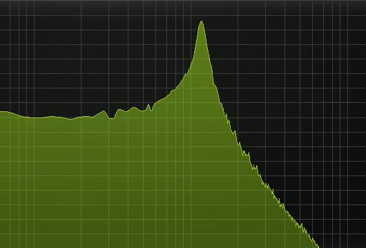
    The Steiner-Parker filter is based on the Sallen-Key topology for 2nd-order active filters. Changing the values of the resistors (see the sketch) can modify the cutoff frequency and resonance.

    It's important to note that this tutorial does not aim to delve into circuit theory or detailed discussions on numerical solvers. If you're interested in configuring Mathematica for circuit-solving purposes, feel free to reach out with your questions. 

    The first thing we need to do is extract the equations. In this case, we have two components with memory (capacitors), so we need to obtain the derivative of the voltage in each capacitor in terms of the input and voltage across the capacitors. In total, we have as many differential equations as there are memory components. Additionally, we need to obtain the output equation.

    To solve this system, the simplest approach is to use the Euler method. However, for a more stable implementation, it is recommended to use the Heun Method (Improved Euler) or Runge-Kutta methods. In the following implementation, I use the Heun Method.

 

Circuit differential equations

\[\frac{d Vc_{1}}{dt} (Input, Vc_{1},Vc_{2},Cutoff,Resonance)\]

\[\frac{d Vc_{2}}{dt} (Input, Vc_{1},Vc_{2},Cutoff,Resonance)\]

\[Output (Input, Vc_{1},Vc_{2},Cutoff,Resonance)\]

 Iterative solution using Heun method

    The Heun method, also known as the Improved Euler method, is a numerical technique used for solving ordinary differential equations (ODEs). It's an iterative approach that refines the predictions made by the Euler method. In each step, it estimates the slope at the current point and uses this information to project the solution forward. Note that in this case, we have a second-order system due to the two capacitors. In the repository, it can be clearly seen how it was implemented.

\[k_{1}=f(t_{n},y_{n})\]

\[k_{2}=f(t_{n}+h,y_{n}+h*k_{1})\]

\[y_{n+1}=y_{n}+\frac{1}{2}h(k_{1}+k_{2})\]

    Where \(h\) is the step size, in this case equals to \(Ts\) (sampling period) / 2.

    Note that in this case, we have a second-order system due to the two capacitors. In the repository, it can be clearly seen how it was implemented. In upcoming posts, we will see how to implement a phaser using the same method.

    Thank you for reading!